

Next: Conclusion
Up: Simulation Results
Previous: Fixed Detector Examples
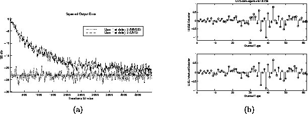
- LMS convergence to the MMSE detector: In single user
applications, the LMS property of converging to the MMSE solution is
what makes the algorithm desirable. This example shows that the
LMS algorithm still converges to the MMSE detector in the multiuser
case. A step size of
 and 100% training bandwidth were used
to generate figure 5.6. The
algorithm does not converge exactly to the MMSE detector because of the
excess MSE caused by the large step size and the fact that the noise
power is 30 dB. Table 5.6 displays the other
parameter settings.

Figure 5.6: (a) Square Output Error trajectory (b) MMSE Detector
Impulse responses

Table 5.6: Parameters for LMS Convergence to the MMSE Detector
- Effects of Power Distribution on Convergence Rates:
Figure 5.7 shows the squared output error of three
different users. Each of the three users has a different amount of
power, which is reflected in the corresponding achievable minimum
MSE. If we look at the initial slope of each of the three users'
squared output error trajectories, we can see a noticeable variance.
It seems that the highest power user has the largest initial slope,
converging close to the MMSE quickly. As the user power decreases,
there is a noticeable decline in the initial convergence rate. This
would lead me to believe that higher powered users have a larger
initial convergence rate. However, there is not enough information to make an
educated decision about overall convergence rate of the different
users. The overall convergence rate depends on the initialization as
well as other system dynamics. Monte Carlo simulations may produce
more conclusive results about the overall convergence rate of
the individual users. Table 5.7 shows the other
selected parameters for the simulation.

Figure 5.7: (a) Square Output Error trajectories (b) Power Distribution
of in cell users. The filled circles correspond with the
trajectories in (a).

Table 5.7: Parameters for Power Distribution Effects on Convergence of LMS
- Effects of Training Bandwidth on Convergence Rate:
When the training bandwidth is varied, we can see the
different effects it has on powerful users and weak users. The plots
in figure 5.8 show the differences for two users
separated by approximately 6dB. For the lower powered user, a 1%
training bandwidth results in very slow convergence in this
particular example. After 5000 iterations the SE is not even -5dB,
which on average corresponds to an undesirable bit error rate.
It appears that if a user has a high SNR, then a reduction in
bandwidth will not affect the bit error rate as much as the lower powered
user, however the initial convergence rate is adversely affected.
The overall effect of training bandwidth will again depend on the
system dynamics. For average performance, Monte Carlo
simulations are necessary. Table 5.8 shows the other
system parameters for this simulation.

Figure 5.8: (a) Square Output Error trajectories for User 1 @ 6dB (b) Square Output Error trajectories for User 3 @ 0dB

Table 5.8: Parameters for Power Distribution Effects on Convergence of
LMS under different training bandwidths
- Near-Far Resistant Minimum Entropy Initialization of CMA:
The initialization technique for CMA presented in [9] is
based on a pre-whitening of the received data to eliminate near-far
effects. Near-far effects cause CMA minima to become very small or
disappear. This is an example showing what happens when the
initialization technique is used for pre-whitened and
non-pre-whitened CMA. I chose a user that was -3 dB from the mean
power of in cell users. Figure 5.9 shows the squared
error tap trajectories for both the whitened and non-whitened
implementations. Both were initialized according to the minimum
entropy initialization scheme, but CMA was run on the whitened and
non-whitened received data respectively. Also shown is the kurtosis
measure for both the non-whitened and pre-whitened initialization.
From this figure we can see that by pre-whitening, we have
initialized in the correct location. (Note: The solid stem is the
desired choice of delay in the Kurtosis plots. Notice that it
corresponds to the largest value in the pre-whitened case, but not
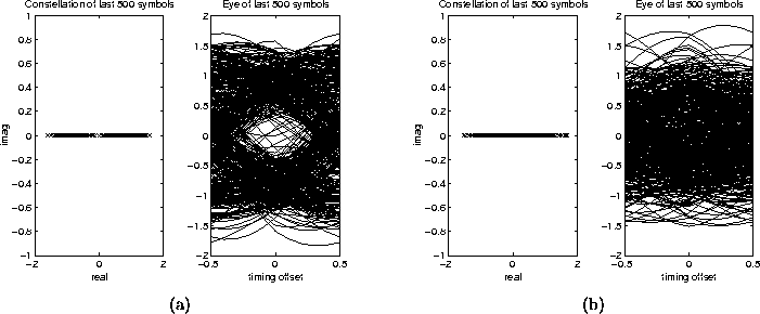
in the non-whitened case.) We can see by figure
5.10 that the eye is opened in the pre-whitened case and
not in the non-whitened case. A Decision Directed algorithm could be
implemented along with the pre-whitened CMA to achieve MMSE like
performance.

Figure 5.9: (a) Square Output Error trajectories for whitened and
non-whitened CMA (b) Kurtosis Measure and Power Distribution

Figure 5.10: (a) Constellation and Eye Diagram for Pre-whitened CMA (b)
Constellation and Eye Diagram for Non-whitened CMA

Table 5.9: Parameters for Whitened vs. Non-Whitened CMA


Next: Conclusion
Up: Simulation Results
Previous: Fixed Detector Examples
Thu Dec 17 13:13:15 EST 1998


